
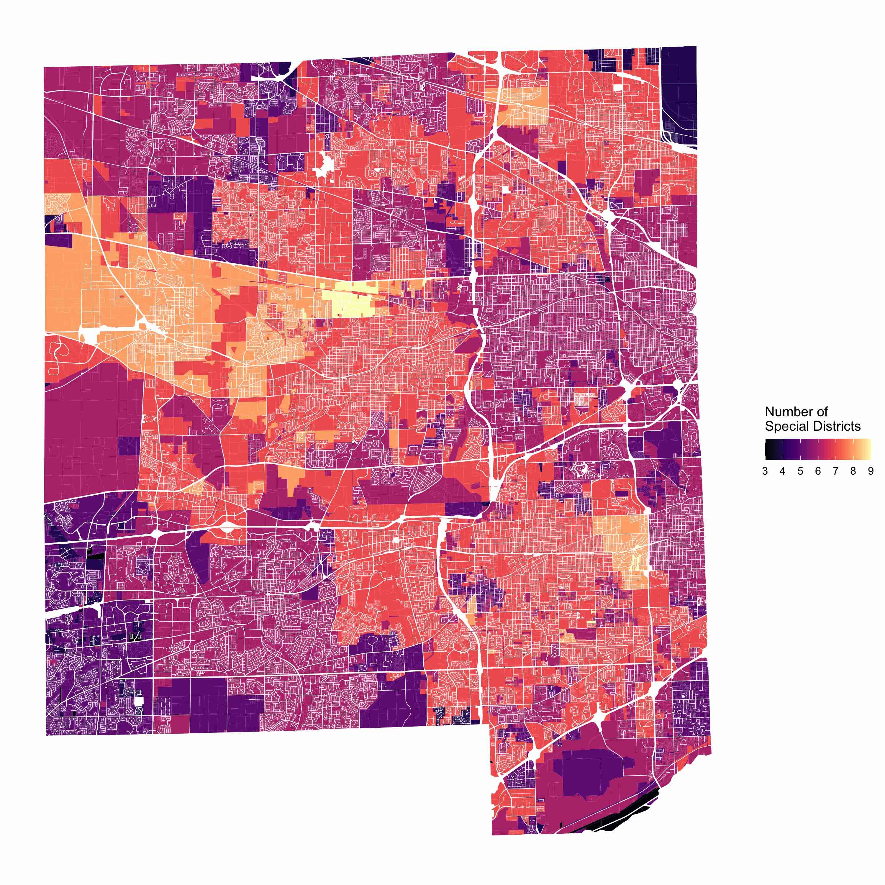
Local governments in the United States generally overlap other local governments. It’s a feature of U.S.-styled federalism that’s difficult to escape. It similarly presents problems for researchers in demonstrating the exact extent of such overlap. Commonly, one might make a map that demonstrates the number of overlapping local governments aggregated by some base geography like a city or a parcel (see right). These are ok; however, they don’t demonstrate how local government borders can be quite eccentric. The borders get lost in the sea of other overlapping governments. We need another method of visualization.
One such method is to rely on 3D visualization methods vs 2D methods. Since local governments overlap, there is a ready made case for separating the layers vertically to demonstrate how each layer differs from the one below. Unfortunately, this is somewhat difficult because map layers are meant to operate in 2D space. Enter the tilting function.
The tilting function
Original function created by Stefan Jünger.
# Function to tilt sf
rotate_sf <- function(data, x_add = 0, y_add = 0) {

  shear_matrix <- function (x) {
    matrix(c(2, 1.2, 0, 1), 2, 2)
  }

  rotate_matrix <- function(x) {
    matrix(c(cos(x), sin(x), -sin(x), cos(x)), 2, 2)
  }

  data %>%
    dplyr::mutate(
      geometry =
        .$geometry * shear_matrix() * rotate_matrix(pi / 20) + c(x_add, y_add)
    )
}
The function essentially tilts the map layer and rotates it off-axis. Then we can arrange each layer on top of one another. See Stefan’s post for more technical details on what the function is doing mathematically. Importantly, the x_add = 0, y_add = 0 options allow us to offset map layers in the x or y directions. I use this extensively in creating the map below.
Creating the map
The visualization of geospatial data has become almost trivial with ggplot and sf in R. We’ll need those packages to begin.
library(tidyverse)
library(sf)
library(ggnewscale)
Load data
The example here uses shapefiles from DuPage County, IL. Illinois has the most independent local governments of any state in the U.S., making this a good test case. Additionally, DuPage County publishes excellent geospatial data on local governments within its borders. They can all be found at DuPage County GIS. I load a subset of such data as a demonstration; however, you can use nearly any sf compatible map layer.
# import parcel database ----------------
parcels = st_read("~/Dropbox/Data/Spatial Data/Dupage/ParcelsRealEstate/ParcelsRealEstate.shp") %>%
  st_union() %>%
  st_sf()

# import townships ----------------
towns = st_read("~/Dropbox/Data/Spatial Data/Dupage/Townships_(PLSS)/Townships.shp")

# import municipalities ----------------
cities = st_read("~/Dropbox/Data/Spatial Data/Dupage/Municipalities/Municipalities.shp") %>%
  filter(CITY != "Uninc")

# import unit school districts ----------------
unit_sd = st_read("~/Dropbox/Data/Spatial Data/Dupage/Unit_School_Districts/Unit_School_Districts.shp")

# import high school districts ----------------
high_sd = st_read("~/Dropbox/Data/Spatial Data/Dupage/High_School_Districts/High_School_Districts.shp")

# import grade school districts ----------------
grade_sd = st_read("~/Dropbox/Data/Spatial Data/Dupage/Grade_School_Districts/Grade_School_Districts.shp")

# import fire protection districts ----------------
fpd = st_read("~/Dropbox/Data/Spatial Data/Dupage/Fire_Protection_Districts/Fire_Protection_Districts.shp")

# import fire protection districts ----------------
lib = st_read("~/Dropbox/Data/Spatial Data/Dupage/Library_Districts/Library_Districts.shp")

# import park districts ----------------
parks = st_read("~/Dropbox/Data/Spatial Data/Dupage/Park_Districts/Park_Districts.shp")
Much of this is run of the mill; however, there are two important bits here. First, I collapse the parcel dataset down to one single polygon using st_union() and make it sf-compatable with st_sf(). This reduces the complexity of the layer and the computation load it takes to render it. You might want to use a terrain raster or some other base map. The parcel map includes the transportation network in the negative spaces, so it is a information-rich base layer. Second, I filter out the unincorporated area polygon from the cities layer. This is useful for identifying which areas are unincorporated; however, I don’t need that information, so it’s filtered out.
Render
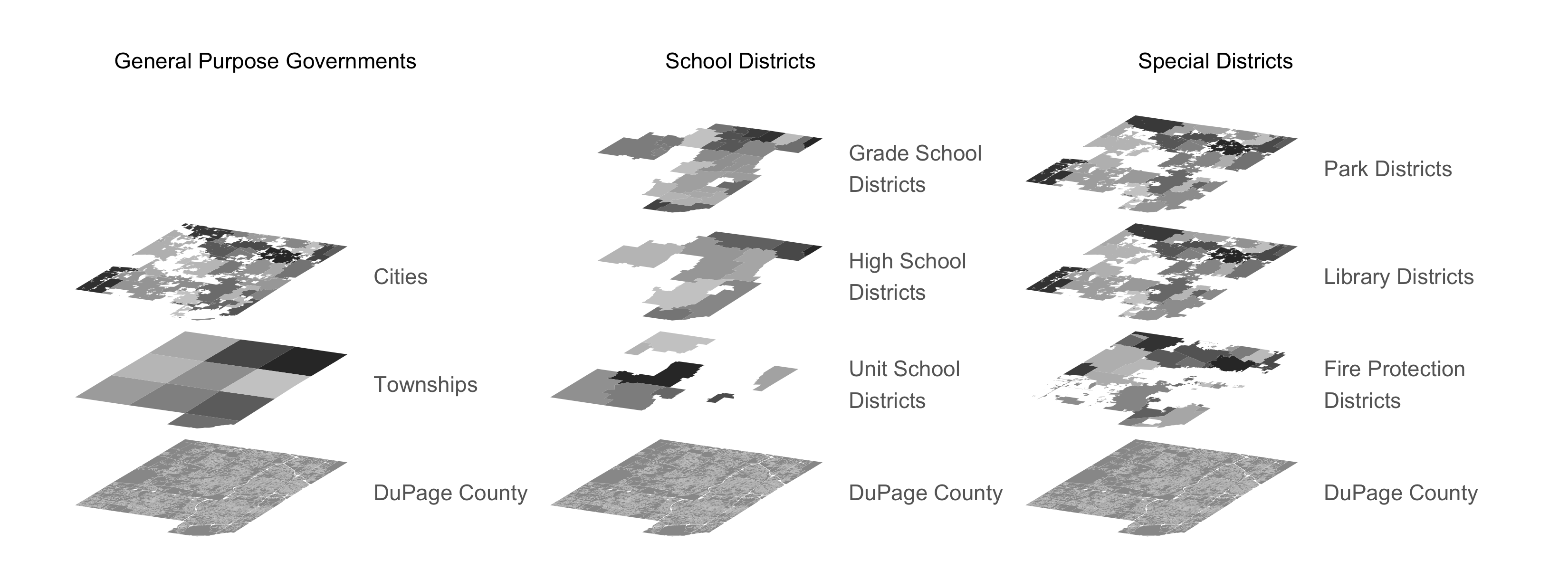
The process here is relatively straightforward. I render each layer, running each data source through the rotate_sf function, and use the x_add = 0, y_add = 0 offset options to create a horizontally and vertically tiled map. The offset parameters rely on the units the map projection uses. This will change depending on how your data are projected.
### plot  ----------------

x = 4800000
color = "gray40"
column2offset = 550000
column3offset = 1100000

p <- ggplot() +
  ### general purpose local government
  ### county base layer
  geom_sf(data = rotate_sf(parcels), color = NA, fill = "gray60", show.legend = FALSE) +
  annotate("text", label='DuPage County', x=x, y=1175000, hjust = 0, color=color) +
  annotate("text", label='General Purpose Governments', x=(x-125000), y=(1550000+125000), hjust = 0.5, color="black") +
  annotate("text", label='School Districts', x=(x+column2offset-125000), y=(1550000+125000), hjust = 0.5, color="black") +
  annotate("text", label='Special Districts', x=(x+column3offset-125000), y=(1550000+125000), hjust = 0.5, color="black") +
  # townships
  new_scale_fill() +
  new_scale_color() +
  geom_sf(data = rotate_sf(towns, y_add = 125000),
          aes(fill = TOWNSHIP_N), color=NA, show.legend = FALSE) +
  scale_fill_grey(aesthetics = "fill") +
  annotate("text", label='Townships', x=x, y=1300000, hjust = 0, color=color) +
  # cities
  new_scale_fill() +
  new_scale_color() +
  geom_sf(data = rotate_sf(cities, y_add = 250000),
          aes(fill = CITY), color=NA, show.legend = FALSE) +
  scale_fill_grey(aesthetics = "fill") +
  annotate("text", label='Cities', x=x, y=1425000, hjust = 0, color=color) +

  ### school districts
  ### county base layer
  geom_sf(data = rotate_sf(parcels, x_add = column2offset), color = NA, fill = "gray60", show.legend = FALSE) +
  annotate("text", label='DuPage County', x=(x+column2offset), y=1175000, hjust = 0, color=color) +
  # unit school districts
  new_scale_fill() +
  new_scale_color() +
  geom_sf(data = rotate_sf(unit_sd, x_add = column2offset, y_add = 125000),
          aes(fill = UNIT_SCHOO), color=NA, show.legend = FALSE) +
  scale_fill_grey(aesthetics = "fill") +
  annotate("text", label='Unit School \nDistricts', x=(x+column2offset), y=1300000, hjust = 0, color=color) +
  # high school districts
  new_scale_fill() +
  new_scale_color() +
  geom_sf(data = rotate_sf(high_sd, x_add = column2offset, y_add = 250000),
          aes(fill = HIGH_SCHOO), color=NA, show.legend = FALSE) +
  scale_fill_grey(aesthetics = "fill") +
  annotate("text", label='High School \nDistricts', x=(x+column2offset), y=1425000, hjust = 0, color=color) +
  # grade school districts
  new_scale_fill() +
  new_scale_color() +
  geom_sf(data = rotate_sf(grade_sd, x_add = column2offset, y_add = 375000),
          aes(fill = GRADE_SCHO), color=NA, show.legend = FALSE) +
  scale_fill_grey(aesthetics = "fill") +
  annotate("text", label='Grade School \nDistricts', x=(x+column2offset), y=1550000, hjust = 0, color=color) +

  ### special districts
  ### county base layer
  geom_sf(data = rotate_sf(parcels, x_add = column3offset), color = NA, fill = "gray60", show.legend = FALSE) +
  annotate("text", label='DuPage County', x=(x+column3offset), y=1175000, hjust = 0, color=color) +
  # fire protection districts
  new_scale_fill() +
  new_scale_color() +
  geom_sf(data = rotate_sf(fpd, x_add = column3offset, y_add = 125000),
          aes(fill = FIRE), color=NA, show.legend = FALSE) +
  scale_fill_grey(aesthetics = "fill") +
  annotate("text", label='Fire Protection \nDistricts', x=(x+column3offset), y=1300000, hjust = 0, color=color) +
  # library districts
  new_scale_fill() +
  new_scale_color() +
  geom_sf(data = rotate_sf(lib, x_add = column3offset, y_add = 250000),
          aes(fill = LIBRARY), color=NA, show.legend = FALSE) +
  scale_fill_grey(aesthetics = "fill") +
  annotate("text", label='Library Districts', x=(x+column3offset), y=1425000, hjust = 0, color=color) +
  # park districts
  new_scale_fill() +
  new_scale_color() +
  geom_sf(data = rotate_sf(lib, x_add = column3offset, y_add = 375000),
          aes(fill = LIBRARY), color=NA, show.legend = FALSE) +
  scale_fill_grey(aesthetics = "fill") +
  annotate("text", label='Park Districts', x=(x+column3offset), y=1550000, hjust = 0, color=color) +
  theme_void(base_family = "Open Sans Condensed Light") +
  scale_x_continuous(limits = c(4450000, 6100000))
All that’s left is to export.
ggsave(p, filename = "./output/layers.png", width=11, height=7.5, units="in", dpi=300, device = grDevices::png, bg = "#ffffff")Concluding thoughts
Local governments in the U.S. are arranged in a complex manner, and showing that complexity is difficult. I present one method of reducing the difficulty of visualization while keeping significant information about the complexity of local government boundaries. Both the number of layers and the relationship between the layers are important.
On a more personal note, creating a map like this has been a bucket list item for a long time. I even considered hiring a graphic designer to make such a map. I am beyond happy that this is easily achievable in R, and that’s largely thanks to Stefan.