
Created in with ggplot2. The relevant code is below.
library(tidyverse)
# read in data
council <- read.csv("citycouncil.csv")
# calculate councilors per 100,000 population
council$pc.council <- council$council/(council$pop17/100000)
# create annotation
annot <- read.table(text=
"city|number|just|text
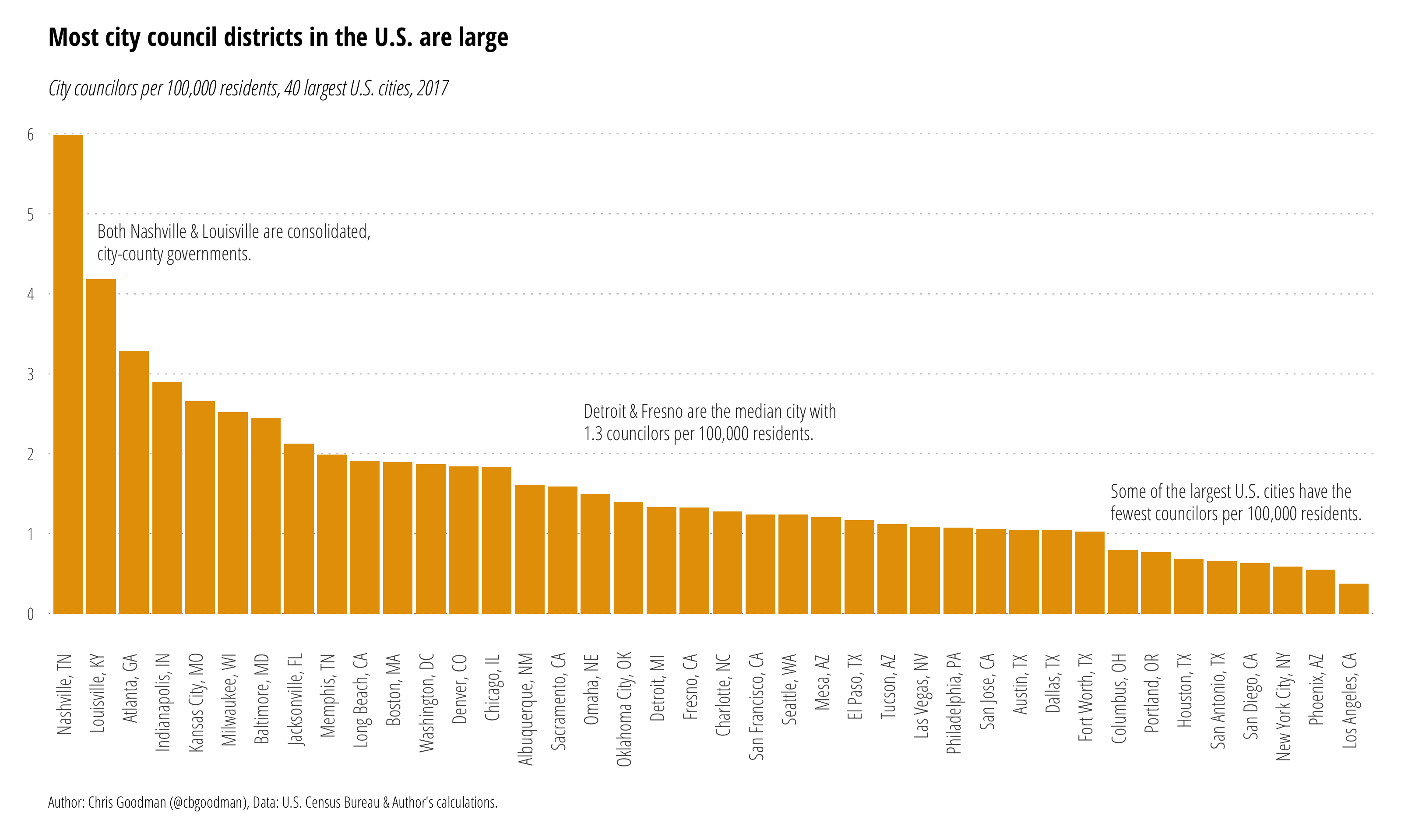
1.75|4.65|0|Both Nashville & Louisville are consolidated,<br>city-county governments.
16.5|2.4|0|Detroit & Fresno are the median city with<br>1.3 councilors per 100,000 residents.
32.5|1.4|0|Some of the largest U.S. cities have the<br>fewest councilors per 100,000 residents.",
sep="|", header=TRUE, stringsAsFactors=FALSE)
annot$text <- gsub("<br>", "\n", annot$text)
# plot
p <- ggplot(data=council,
aes(x=reorder(City, -pc.council), y=pc.council, width=0.9))+
geom_bar(stat="identity", fill="#E69F00")+
#geom_bar(stat="identity", fill="#999999")+
scale_y_continuous(breaks=seq(0, 6, by=1))+
# read in annotations
geom_label(data=annot, aes(x=city, y=number, label=text, hjust=just),
family="Open Sans Condensed Light", lineheight=0.95,
size=3.5, label.size=0, color="#2b2b2b")+
# Theming
labs(
title="Most city council districts in the U.S. are large",
subtitle="City councilors per 100,000 residents, 40 largest U.S. cities, 2017",
caption="Author: Chris Goodman (@cbgoodman), Data: U.S. Census Bureau & Author's calculations.",
y=NULL,
x=NULL) +
theme_minimal(base_family="Open Sans Condensed Light") +
# light, dotted major y-grid lines only
theme(panel.grid=element_line())+
theme(panel.grid.major.y=element_line(color="#2b2b2b", linetype="dotted", size=0.15))+
theme(panel.grid.major.x=element_blank())+
theme(panel.grid.minor.x=element_blank())+
theme(panel.grid.minor.y=element_blank())+
# light x-axis line only
theme(axis.line=element_line())+
theme(axis.line.y=element_blank())+
theme(axis.line.x=element_blank())+
# tick styling
theme(axis.ticks=element_line())+
theme(axis.ticks.x=element_blank())+
theme(axis.ticks.y=element_blank())+
theme(axis.ticks.length=unit(5, "pt"))+
# x-axis labels
theme(axis.text.x=element_text(size=10, angle=90, hjust=0.95,vjust=0.2))+
# breathing room for the plot
theme(plot.margin=unit(rep(0.5, 4), "cm"))+
# move the y-axis tick labels over a bit
#theme(axis.text.y=element_text(margin=margin(r=-5)))+
# make the plot title bold and modify the bottom margin a bit
theme(plot.title=element_text(family="Open Sans Condensed Bold", margin=margin(b=15)))+
# make the subtitle italic
theme(plot.subtitle=element_text(family="Open Sans Condensed Light Italic"))+
theme(plot.caption=element_text(size=8, hjust=0, margin=margin(t=15)))
ggsave(plot=p, "councilors.png", width=10, height=6, units="in", dpi="retina")Full code and data can be found here.